More on fixing the little white lines

 The basic problem we are having with the strips for the second Gordo book is that some of the images (particularly the odd-page numbers, which would be the right-hand side images -- the backs of the pages), were copied on a machine which introduced thin white lines across the images.

If we look at an image, and blow it up we find:

In this small segment of an image, we can see 4 white lines.  The green pixels are ones that our programs have identified and marked as being white, but should be black.   A lot of the green pixels are just single pixel errors -- general noise -- and not associated with the white lines explicitly.

We have tried for months to write programs that will find just the white lines and fill them in.  It seems at first to be relatively simple:  look for white pixels with black pixels above and below.  But consider the following image segment:

This would seem to be an obvious case of a thin (3 pixel) white line.  But if we pull back from this and look at the larger context,

The gap in the previous image is the space between the bottom of one A and the top of the A on the next line.  It is not something that should be fixed.  Although, it may in fact actually be a 3-pixel white line that just happened to be in exactly that place; it requires judgement to determine if it should be filled in or not.

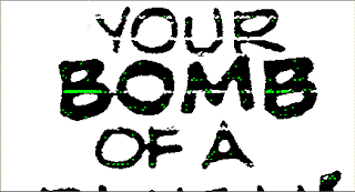
And there are lots of places in the images where there are a "small" number of white pixels have black above and below, but are not caused by a white line.  Consider in the original image we showed above

 The space between the top line of the F and the middle line should not be filled in, but meets the simple definition -- a small number of white pixels with black above and below.  The letter E is an even worse case.

So after months of trying to program fixing the lines, it seemed that I needed to just do it by hand.  On my Linux system, the image editor GIMP provides me the ability to edit images one pixel at a time.  So I just need to load each image and then find the little white lines, and change the appropriate white pixels to black. 

Of course that would be tedious at best.  Pixel by pixel editing is very time consuming.  We want to be able to see what we have changed and what was the original image, so we change the pixels from white to green, and then can use a later program to change the green pixels to black.  We use a pencil setting to draw green pixels over the white pixels that we want to change.

And to avoid having to change just exactly the right (white) pixels,  we developed a process that allows us to draw slightly out of the lines and also change black pixels.  A program then compares the modified image with the original image and if it finds a green pixel where there used to be a black pixel, it keeps that pixel black, remembering the green pixel only if the previous pixel was white.  This allows us to be a bit sloppy in our editing so we can work faster.

So if we take our example image, we can mark it as:

and then process it down to 

We are working on each panel of the book, one at a time.  We started this in May, and it looks like we may finish it by November or December.

Understanding the Hough Transform

 Our basic code to find the white lines that the photocopying process has introduced is to use a Hough Transform, which we described in a previous post "Fixing the Photocopy Lines".  But we are having a number of problems with our code for that use.  So let us try to understand Hough Transforms and how they work better.

Let us start with a really simple case: a simple  48 pixel long well-defined perfectly horizontal line (from (5,16) to (52,16)).

If we feed this into our Hough Transform code and look at the matrix that is produced by it, we find it looks like:

The maximum value (48) is right in the middle of row 16, corresponding to a slope of 0 and an intercept of 16.  But we also compute for lines that go thru each point of the line for 31 different slopes, each a tiny bit different from the previous (both positive and negative).

So although the maximum is a slope of 0 and an intercept of 16, we also have the same maximum for a slope slightly less and slightly more (a slope so that at the end of the image, the line would be one pixel higher or lower, so not quite level).  This is because of the integer arithmetic used.  As the slope gets higher (or lower), some pixels will actually intercept the edge of the image higher and lower.  Notice that the sum in each column (sum over all slopes) is 48, since all 48 green pixels contribute to some b-intercept line, for each different slope.

If the green line gets thicker, then there are multiple intercepts for the thicker line (from 15 to 17, for example for a 3-pixel wide line), and the Hough transform matrix expands similarly.

Note that each column still adds up to 48 (times 3 now that we have 3 lines of 48 green pixels).  But the maximum value (48) occurs 15 times -- five times on each of the 3 lines for the intercept lines corresponding to the 3 straight, horizontal lines.

And we start to see other local maximums, for example the 39 up one line from the 3 real intercepts, and to the left and right of the center.  This probably corresponds to a line that would start at the lower of the 3 lines at the left and then move right into the center line and up to the upper line, exiting at the right-most pixel of the upper line.  And a similar line going down from the left-most green pixel for the upper line to the right-most green pixel for the lower line. 

So while a maximum value in the Hough Transform matrix corresponds to a particular slope/intercept line, there may be multiple maximums suggesting a thicker line.

In a noisy environment, however, we would expect that there are no perfect lines.  For a perfectly horizontal single-pixel line, that would mean a lower maximum -- some of the pixels that "should" contribute to it are missing -- but we would still expect that the maximum is larger than the lower values in the matrix. 

If we poke holes in the lines, corresponding to noise, we can end up with more or fewer non-green holes in each of the 3 lines corresponding to the width of the line, and higher or lower values in the Hough Transform matrix.  For example, putting one non-green pixel in the lowest line, five in the central line, and 3 in the upper line, moves the maximum to 47 in the line corresponding to the lowest line, 43 for the line corresponding to the middle line, and 45 in the upper line.   This gives a cluster of values from from 47 to 43, and then a drop to 38, 37 ... and much lower values.  But it is not clear how to differentiate between the 43 (which is 4 below the maximum) ad the 38 (which is only 5 below that)

But there could be other high-value entries "close" to the maximum that correspond to a thicker line -- not just one pixel.

If we look at a real example, panel p027_1_1, we find the maximum at 783,22 with a value of 276.  There is a 274,  at 784,20, and a 239 at 785,18.  We have to drop to 182 to get away from the cluster of high numbers in rows 784 to 790.

Panel Borders

Most of the panels have borders -- a line box drawn around the contents of the panel. So it seems that we should be able to recognize the border as a black line of some thickness, and fill in any missing pixels -- white pixels in the black border.

In particular, for those pages with little white lines from the copying process, if we find a set of white pixels on the left and the right, it suggests there is a little white line connecting them.  That could help us repair those lines.

So the first problem is to recognize the border, where it is in the panel and it's thickness. There are four sides to a panel: left, top, right, and bottom.  The border should run along the outside next each of these sides, as a continuous line of black pixels.

Except the border, as with all the art of the panels, was hand drawn, so it's not perfectly straight and uniform.  We could, if we can recognize it, adjust it so that it was in fact a perfectly straight line of uniform width on all sides.  But that would change the nature of the panel, and we don't want to do that; we want to maintain the hand-drawn nature of the borders.

So we wrote code that will scan, starting from the outside edge over any white pixels, until we find the black pixels that make up the border, and then scan over those black pixels to find the other side of the border, giving us the location and width of the border.  Trying to match this simple model of the border reveals several problems:

(1) Not all panels have borders.  For example, p152_1_3 has no border.

Turns out there are a lot of our panels that do not have borders.  This is especially true at the very beginning, where each letter of a large title is a "panel" and none of them have borders. 

 

(2) Not all panels stay inside the borders.  For example, p016_3_3, so we may find stuff before the border, and the border may be interrupted by art work laying "on top" of the border. 

(3) Some of our "panels" are not just one panel.  For example, p150_4_2 is actually two panels with a word balloon that spans between them, over the "gutter" between them. 

(4) Notice that we then also have to allow for "gaps" in the border.  If we have a file that is one or more panels that cannot be easily separated, such as p146_3_1, the border may not be complete or contiguous. 

 
(5) Arriola has a style of a "panel" of words next to a panel of art instead of a large word balloon.  These word panels do not have borders, and there are a lot of them.

(6) But these word panels are the speech of a particular character and so there is the "tail" of the word balloon pointing at the character doing the speaking.  This tail consists of a sidways V that pierces the border and points to the speaker.  See for example, p010_3_3 and the following art panel p010_3_4.  These V shaped tails can be on either the left or the right. 

 

(7) This latter art panel, p010_3_4, also illustrates that the borders may have strange corners and ticks, as illustrated in the lower left corner.  

 

Sometimes it is even more extreme, like p012_2_4 which has a noticeable corner tick in both the upper right and lower right. 

(8) The border may run into the art.  Consider p041_3_1 which shows the two characters in silhouette against a porthole.  The "border" is obvious on the top, but as it runs down the sides and across the bottom is merged directly into the art.
 

(9) Some panels may be both borderless text and an art panel together, for example, p041_2_2.  This is similar to point (3) above.

 

So first we try to isolate and identify those panels that are simply rectangles with solid borders.  Well except for the V shape gaps for the tail of a word panel. This produces a list of 1276 panels.  This should allow us to find the average width of the borders when it is there.

Doing this, and then looking at the computed border widths, shows that they peak at about 19 pixels in width, largely between 15 and 26 pixels. 

Except for a smaller peak at 3 or 4 pixels.  For example, p043_3_1 has a left border of 3, a top border of 3, a right border of 4, and a bottom border of 7.  

 

 

Of course these numbers are only a summary.  The borders vary from 1 to 429 because of effects such as (8) above where the border and the art run together.  For example in p043_3_1, the right and bottom borders merge with the hair of the one character in the lower right.  The top border, on the other hand is not affected by these problems, but even it runs from 1 pixel in spots to 11 in another.  The histogram of the various widths shows:

  1  81
  2  319
  3  335
  4  238
  5  225
  6  166
  7  134
  8  64
  9  6
10  4
11  1

So the most common width is 4, but anywhere from 2 to 5 (possibly 7) is pretty much the same.

(This particular part of the book is describing a time travel story and maybe the thinner border is a reflection that these events are in the past.)

So we adopt the definition that the border starts with the first black pixel and is at most 20 to 22 pixels wide, but may be shorter.

Another property that we would expect is that, at the 600 dpi that we are scanning the images, the border, while it may vary, will not vary by very much from one scan line to the next.  We would expect it to often be the same, or maybe more one or two pixels either direction.  If we look at where the border begins, and then at where it begins for the next row or column, and look at the histogram of the difference between those two, we get numbers that vary from -89 to +58, but the peak (5,345,976) is at zero, and by plus/minus 3, is down to about 6,000.

Look at the histogram of differences. 

We can use the outliers to identify issues with the panels.  For example, the 58 value corresponds to p081_3_3, and shows that the quotes that belong in the following text panel have been incorrectly put in this panel.  

 

If we pick those values that are plus/minus 20 pixels or more, we get a selection of 144 panels to examine. Making it plus/minus 30 reduces this to just 28.  For example, checking p025_2_1 which has a value of -30 on the bottom, we find it is caused by a dust speck on the bottom of the panel, which we remove. 

While, we are looking at p025_2_1, we notice that it seems skewed. If you follow the border from left to right, across the top, it drops about 17 pixels, 20 pixels on the right, 13 pixels across the bottom, and 24 on the left.  This suggests that it is skewed -- not aligned to the page that it is on, but slightly rotated.

We can check for skew by using the outer set of pixels that define the border to define a line that is the linear least squares best fit for the border.  We can then compare the slopes for the four sides and if we find they are all or the same sign and roughly the same magnitude, then it suggests that the image is skewed. 

images1/p025_2_1.gif:   left border is slope -0.018, intercept    25.58
images1/p025_2_1.gif: bottom border is slope -0.009, intercept    32.83
images1/p025_2_1.gif:  right border is slope -0.013, intercept    22.73 images1/p025_2_1.gif:    top border is slope -0.012, intercept    18.21
images1/p025_2_1.gif: min slope=-0.018;max slope=-0.009;diff slope= 0.009 ###


That is not technically correct, since obviously the top and bottom sides are perpendicular to the left and right.  However our code is written to only work on one side -- the left side of the panel.  To get the top, right, and bottom sides, we rotate the original panel 90 degrees, and then run our code again.  Rotate again for the right; rotate again for the top. This makes the computations for each side the same and gives comparitive numbers for any of the statistics, like the slopes.

This rotation approach causes one difficulty.  If we have rotated the image 90 degrees, then what the program is seeing as location (i,j) in the image is not what I see as (i,j) in the image. If we are printing the location of a pixel, we want to see it in its true position, not in it's rotated position.

In particular, if we compute a line that approximates each border, we should be able to compute the intersection of the lines for the left side and the top side to compute the corner pixel that defines where we should start working on the image -- we don't want to process the background that exists outside the border.  But this is more difficult because the lines for the top and the left sides have been computed in different coordinate systems and will need to be translated to the true coordinate system to identify the spot where they intersect.

Fixing the Photocopy Lines, Part 2

 We have spent months, literally months, trying to fix the code that uses a Hough transform to find the little white lines introduced by the photocopying process and have more problems than we anticipated.   First our code does not find all the white lines, and second it finds lines where there are no lines.

The first problem seems to be because there are lots of potential white lines, since there are so many white pixels.  The second is that some parts of the images seem to be just so that, in isolation, they can be interpreted as being part of a white line, when they are not.

But in working with the images,  I noticed that if you look at the lines so that you can see the individual pixels, like:

You can see that the white lines tend to be represented by small groups of disconnected white pixels.  It is only when you get a really big white line that you get long sections of white pixels.  And the small groups of pixels seem to be in repeating patterns. For example in the above image, the last group of pixels in the last line is repeated earlier in that line, as well as in the line above it.

So it looks like, if we scan the images for small groups of white pixels -- say something that would fit in an 8x8 square, and count how many times those patterns are repeated in the images, then we can take the most common ones and when we find them in an image, fill them n with black.

In fact we can use the partially fixed images from using the Hough transform and diff them with the original images to get just bits that we believe are in little white lines.  From that we can produce a list of the most frequent patterns, and then use those patterns on the original images to find a larger set of little white lines.

Writing a program to find the patterns, produces thousands of potential patterns, but looking at the frequencies, most patterns occur in just a few places -- less than 10.  There are 776 patterns of more than 10 occurrences, and they are no bigger than 7x7.

A second program can find those patterns.  The pattern is all white, but we believe it should be black.  To observe what we are finding, we set the pixels to green.  This produces an output file like:

Notice that a lot of the previous white lines have been filled in.  Not all of the line is filled in, since we are requiring each pattern to be white pixels surrounded by black pixels.  If the white pixels are too close, we do not replace them.  And if the white line is just too big, we don't find anything at all.  And if the white line goes thru a vertical black line, just leaving a gap in the black line, we miss that too.

But if we now use these green pixels to drive a Hough transform, we may be able to better identify the lines, and then go back and fill in the missing white pixels.  We will try that next.

Oh, and if we just count the number of green pixels on a page and plot that, ordered by the number of pixels, tagging each file with it's file name, it becomes clear that the problem is almost exclusively with the odd pages (the back sides) and not the even pages.

The sudden jump in the number of green pixels is from 20K green pixels for p128 to 40K green pixels for p019.  All of the even pages are below p128, and all of the odd pages (except one) are above p019.  The exception is p001 which has no green pixels.  p001 is the copyright page, which we had to process by hand to make visible.

But even the even pages can have thousands of green pixels, which when looked at closely show a lower level of the same photocopy problem.  So our techniques will be applied to all the pages.

Fixing the Photocopy Lines

From reading graphics processing books, it appears that fixing the thin little horizontal lines that have been introduced into the images by the photocopying process should be fairly easy.  All we have to do is use a Hough transform.  

A Hough transform is used to find straight lines in an image.  The idea is to look at each pixel and say "if there was a straight line going thru this point, what would it be?".   The equation for a line with slope a and y-intercept b going thru the point (x,y) is y = ax+b.  Now if we have (x,y) and want to solve for a and b, that would be better presented as b = y - ax.  Now give x, y and a we can solve for b.  

A Hough transform defines an accumulator matrix m and stepping thru the possible slopes, a, computes b = y - ax for each allowable a and adds one to the location in the matrix defined by m[a,b].  The idea is that if the line is actually there, all the points along the line will add to m[a,b] for the line with a particular slope a and intercept b.  All the non-lines will just sort of add randomly to other locations in the matrix.  So the matrix locations with large counts correspond to lines and the others are all just noise.

There are problems with this approach when the slope approaches vertical since the slope tends towards infinity, but in our case we are only interested in horizontal (or mostly horizontal) lines.  In fact, we expect that if we limit our work to each panel of a strip, instead of an entire strip, then the skew will be minor and we are actually looking for horizontal lines.  In that case a = 0, and we simply accumulate into a vector m[b] whenever  for a line defined by b = y + 0x or just b = y.

So for each point (x,y) that we think might be on a line, we add one to m[y] and look for the high values of the resulting vector.

So we are interested in a point if it is on a line.  We know the lines look like:

 

So we look for a column with a small number of white pixels with black pixels above and below.  Then we accumulate the number in a particular row, and look for the rows with the largest accumulation.  For a row like that, we then step down it looking for the small cluster of white pixels and setting them all to black.

There are some parameters for this, like how many white pixels in a row, and how many black pixels above and below the white pixels.  We start with up to 5 white pixels and needing 10 black pixels above and below.

As we suspected, the fine white lines mainly show up on the odd numbered files, which would be the left hand pages, which was the "back" of the sheets as they were copied. 

When we use this approach, we find two types of errors.  One is some very noticeable white lines that are not caught. Going thru all 1884 panels, we find 150 that still need work.

Some of those are because the white lines are big than we anticipated.  For example, here on panel 3 of strip 4 on p013, the white line is sometimes 6 pixels high.

Another problem is where we have what we think might be a white line, but is actually part of the original art.  For example in the 2nd panel of the 2nd strip of p034, we have the following art:

Which actually has no white lines in it.  But notice that there are two marks on the plate, just below the top rim.  The distance here between the white and the black is such that my code things this is part of a thin white line, and fills those white pixels in, producing:

So I need to either improve my code, or ferret out all these sorts of problems and fix them by hand. 

Starting the Second Gordo Book

Most of the technical issues for the first Gordo book (Gordo Redux) are handled, so we turn our attention to the second Gordo Book (Gordo Galore). As with the first one we scanned it at 600 dpi. Then we can run the same set of programs we used on the first book, convert the pages from gray scale to black and white, clean up the images, to create the cboxes and pull the individual strips out as images.

But a new problem is presented by this particular book: when it was photocopied at some point, thin white lines were introduced into the copy.  This seems particularly a problem on the backs of the pages, the left-hand sides which would be odd pages.  For example look at part of p029:

I've seen these sorts of lines on Xerox copies for decades.  They are caused by dirty or defective points in the photocopy machinery or toner. 

But we would like to identify these lines, and fill them in with the missing black to restore the original image drawn by Arriola.  

If we expand in and look at the individual pixels, we see that the lines are not constant, but rather a mixture of light and dark pixels.

When we convert this to pure black and white pixels, the picture changes somewhat, but we still have these lines.

It appears that many of these could be detected by simply changing small pieces of white surrounded by black to black, but as with the first book, there some places were that would change the image.  Although for the first book, the image we found which limited us to only clusters of 10 pixels or less was an issue of a black cluster in a white background.

Still there are some places where that would be insufficient.  If we follow the lines shown above to the left in this same image, we get:

At least for the line on the right, the little white channels breaking the otherwise solid vertical line probably should not be filled in without the context of knowing that there is a thin white line crossing the page.

To study this problem, I tried to look at where the white lines are, in this image, by examining the borders for the panels. This image has 3 panels, so a left border, two gutters of white with borders at roughly 1/3 and 2/3 horizontally, and a right border.  If I try to list the white lines at each vertical border, I get:

The largest, most obvious white lines are marked with an "@" symbol.  The numbers represent the starting row of the white line, and the number of pixels high that it is.  So "447,3" is a gap that starts at row 447 and continues to row 449.  There are a couple of things we can note from this chart.

One is that the white lines are not actually strictly horizontal.  As they move from left to right, following a white line, for this image, the row position decreases. So there is skew. The last column shows the difference between the left hand row position and the right hand row position.  For this image it decreases by  a skew of 20 to 27 pixels in the span of 4446 columns, about 0.6%.  But notice also that, at least in this case, the skew is not constant for this image, but seems to decrease, almost uniformly as the row changes.  And since the skew is not constant, it is not a property of the scanning.

And lines do not seem to appear across the entire image.  A line may stop or start in the middle of the image.  From p029, for example:

Here we see a major line towards the bottom that continues thru the image, although varying someone is "strength".  Other lines, at the top, start and stop at intervals.

If we can identify the lines, we can fill them in to change the above image to

Laying out the pages

 In addition to the page numbers on each page (which are separate characters), we have the comic strips themselves.  Mostly we have 4 strips per page, with blank horizontal rows between them. We don't need to keep or regenerate the blank rows.  We have a program that can identify the blank rows between the strips and pull out the strips and make them separate image files. 

Checking the sizes of the images, we find them all between 4050 and 4660 pixels wide and between 1230 and 1320 pixels high.  The actual location on the page varies due to either the original layout by Arriola or the scanning process.  But having isolated each strip, we can position them on the page consistently.  Of course, we need to take account of the left-hand/right-hand nature of each page and make sure we have enough extra room on the inside margin for the binding process.

Standard page layout for an 8.5 x 11 inch piece of paper allows us 1/4 inch for both the left and right margin, plus an extra 1/8 inch for the gutter.  This means we want each page to start horizontally at 150 pixels for a left-hand page and 225 for a right-hand page.  The page would end horizontally at 4950 pixels for a right-hand page and 4875 pixels for a left-hand page.  Since each image, however, is a different size, if we pin down the starting point of an image, we don't control the ending point -- the ending point is determined by the starting point plus the length of the image. 

We have allowed 4875 - 225 = 4650 pixels for each image, but we know most images are less than this.  So we position each image so that it is right-adjusted on a right-hand page, and left-adjusted for a left-hand page.  These leaves any extra space from the image being less than maximum size in the gutter. 

The longest page (ignore the page numbers) is 5808 pixels.  Add the top margin of 300 pixels, and the last panel ends by 6108.  We can put the page numbers so that the baseline is at 6300, centered under the pages (the center being at 2512 pixels for left-hand pages and 2737 for right-hand pages.